Generalized CP (GCP) Tensor Decomposition

>> Tensor Toolbox >> CP Decompositions >> GCP-OPT

This document outlines usage and examples for the generalized CP (GCP) tensor decomposition implmented in gcp_opt. GCP allows alternate objective functions besides sum of squared errors, which is the standard for CP. The code support both dense and sparse input tensors, but the sparse input tensors require randomized optimization methods. For some examples, see also GCP-OPT and Amino Acids Dataset.

GCP is described in greater detail in the manuscripts:

D. Hong, T. G. Kolda, J. A. Duersch, Generalized Canonical Polyadic Tensor Decomposition, SIAM Review, 62:133-163, 2020, https://doi.org/10.1137/18M1203626
T. G. Kolda, D. Hong, Stochastic Gradients for Large-Scale Tensor Decomposition. SIAM J. Mathematics of Data Science, 2:1066-1095, 2020, https://doi.org/10.1137/19m1266265

Basic Usage
Manually specifying the loss function
Choice of Optimzation Method
Specifying Missing or Incomplete Data Using the Mask Option
Other Options
Specifying L-BFGS-B Parameters
Specifying SGD and ADAM Parameters
Example on Gaussian distributed
Boolean tensor.
Create and test a Poisson count tensor.
Loss function for Poisson negative log likelihood with identity link.

Basic Usage

The idea of GCP is to use alternative objective functions. As such, the most important thing to specify is the objective function.

The command M = gcp_opt(X,R,'type',type) computes an estimate of the best rank-|R| generalized CP (GCP) decomposition of the tensor X for the specified generalized loss function specified by type. The input X can be a tensor or sparse tensor. The result M is a Kruskal tensor. Some options for the objective function are:

'binary' - Bernoulli distribution for binary data
'count' - Poisson distribution for count data (see also cp_apr)
'normal' - Gaussian distribution (see also cp_als and cp_opt)
'huber (0.25)' - Similar to Gaussian but robust to outliers
'rayleigh' - Rayleigh distribution for nonnegative data
'gamma' - Gamma distribution for nonnegative data

See Function Types for GCP for a complete list of options.

Manually specifying the loss function

Rather than specifying a type, the user has the option to explicitly specify the objection function, gradient, and lower bounds using the following options:

'func' - Objective function handle, e.g., @(x,m) (m-x).^2
'grad' - Gradient function handle, e.g., @(x,m) 2.*(m-x)
'lower' - Lower bound, e.g., 0 or -Inf

Note that the function must be able to work on vectors of x and m values.

Choice of Optimzation Method

The default optimization method is L-BFGS-B (bound-constrained limited-memory BFGS). To use this, install the third-party software:

L-BFGS-B by Stephen Becker

The L-BFGS-B software can only be used for dense tensors. The other choice is to use a stochastic optimization method, either stochastic gradient descent (SGD) or ADAM. This can be used for dense or sparse tensors.

The command M = gcp_opt(X,R,...,'opt',opt) specifies the optimization method where opt is one of the following strings:

'lbfgsb' - Bound-constrained limited-memory BFGS
'sgd' - Stochastic gradient descent (SGD)
'adam' - Momentum-based SGD method

Each methods has parameters, which are described below.

Specifying Missing or Incomplete Data Using the Mask Option

If some entries of the tensor are unknown, the method can mask off that data during the fitting process. To do so, specify a mask tensor W that is the same size as the data tensor X. The mask tensor should be 1 if the entry in X is known and 0 otherwise. The call is M = gcp_opt(X,R,'type',type','mask',W).

Other Options

A few common options are as follows:

'maxiters' - Maximum number of outer iterations {1000}
'init' - Initialization for factor matrices {|'rand'|}
'printitn' - Print every n iterations; 0 for no printing {1}
'state' - Random state, to re-create the same outcome {[]}

Specifying L-BFGS-B Parameters

In addition to the options above, there are two options used to modify the L-BFGS-B behavior.

'factr' - Tolerance on the change on the objective value. Defaults to 1e7, which is multiplied by machine epsilon.
'pgtol' - Projected gradient tolerance, defaults to 1e-4 times total tensor size.

It can sometimes be useful to increase or decrease pgtol depending on the objective function and size of the tensor.

Specifying SGD and ADAM Parameters

There are a number of parameters that can be adjusted for SGD and ADAM.

Stochastic Gradient. There are three different sampling methods for computing the stochastic gradient:

Uniform - Entries are selected uniformly at random. Default for dense tensors.
Stratified - Zeros and nonzeros are sampled separately, which is recommended for sparse tensors. Default for sparse tensors.
Semi-Stratified - Modification to stratified sampling that avoids rejection sampling for better efficiency at the cost of potentially higher variance.

The options corresponding to these are as follows.

'sampler' - Type of sampling to use for stochastic gradient. Defaults to 'uniform' for dense and 'stratified' for sparse. The third options is 'semi-stratified'.
'gsamp' - Number of samples for stochastic gradient. This should generally be O(sum(sz)*r). For the stratified or semi-stratified sampler, this can be two numbers. The first is the number of nonzero samples and the second is the number of zero samples. If only one number is specified, then this is used as the number for both nonzeros and zeros, and the total number of samples is 2x what is specified.

Estimating the Function. We also use sampling to estimate the function value.

'fsampler' - This can be 'uniform' (default for dense) or 'stratified' (default for sparse) or a custom function handle. The custom function handleis primarily useful in reusing the same sampled elements across different tests. For instance, we might create such a sampler by calling the hidden sampling function and saving its outputs:

[xsubs, xvals, wghts] = tt_sample_uniform(X, 10000);
fsampler = @() deal(xsubs, xvals, wghts);'

'fsamp' - Number of samples to estimate function. This should generally be somewhat large since we want this sample to generate a reliable estimate of the true function value.

The 'stratified' sampler has an extra option: * |'oversample'| - Factor to oversample when implicitly sampling zeros in the sparse case. Defaults to 1.1. Only adjust for very small tensors.

There are some other options that are needed for SGD, the learning rate and a decrease schedule. Our schedule is very simple - we decrease the rate if there is no improvement in the approximate function value after an epoch. After a specified number of decreases ('maxfails'), we quit.

'rate' - Initial learning rate. Defaults to 1e-3.
'decay' - How much to decrease the learning rate once progress stagnates, i.e., no decrease in objective function between epochs. Default to 0.1.
'maxfails' - How many times to decrease the learning rate. Can be zero. Defaults to 1.
'epciters' - Iterations per epoch. Defaults to 1000.
'festtol' - Quit if the function estimate goes below this level. Defaults to -Inf.

There are some options that are specific to ADAM and generally needn't change:

'beta1' - Default to 0.9
'beta2' - Defaults to 0.999
'epsilon' - Defaults to 1e-8

Example on Gaussian distributed

We set up the example with known low-rank structure. Here nc is the rank and sz is the size.

rng('default')
nc1 = 2;
sz1 = [20 30 40];
info1 = create_problem('Size',sz1,'Num_Factors',nc1);
X1 = info1.Data;
M1_true = info1.Soln;

Run GCP-OPT

rng('default')
tic, [M1,M1_0] = gcp_opt(X1,nc1,'type','normal','printitn',10); toc
relfit1 = 1 - norm(X1-full(M1))/norm(X1);
fprintf('Final fit: %e (for comparison to f in CP-ALS)\n',relfit1);
fprintf('Score: %f\n',score(M1,M1_true));

GCP-OPT-LBFGSB (Generalized CP Tensor Decomposition)

Tensor size: 20 x 30 x 40 (24000 total entries)
GCP rank: 2
Generalized function Type: normal
Objective function: @(x,m)(m-x).^2
Gradient function: @(x,m)2.*(m-x)
Lower bound of factor matrices: -Inf
Optimization method: lbfgsb
Max iterations: 1000
Projected gradient tolerance: 2.4

Begin Main loop
Iter    10, f(x) = 2.404359e+03, ||grad||_infty = 4.19e+01
Iter    20, f(x) = 4.732223e+02, ||grad||_infty = 2.32e+02
Iter    30, f(x) = 1.870785e+02, ||grad||_infty = 5.47e+00
Iter    31, f(x) = 1.870410e+02, ||grad||_infty = 8.77e-01
End Main Loop

Final objective: 1.8704e+02
Setup time: 0.00 seconds
Main loop time: 0.02 seconds
Outer iterations: 31
Total iterations: 70
L-BFGS-B Exit message: CONVERGENCE: NORM_OF_PROJECTED_GRADIENT_<=_PGTOL.
Elapsed time is 0.021493 seconds.
Final fit: 9.008914e-01 (for comparison to f in CP-ALS)
Score: 0.998776

Compare to CP-ALS, which should usually be faster

rng('default')
tic, M1b = cp_als(X1,nc1,'init',M1_0,'printitn',1); toc
err1b = norm(X1-full(M1b))^2;
fprintf('Objective function: %e (for comparison to f(x) in GCP-OPT)\n', err1b);
fprintf('Score: %f\n',score(M1b,M1_true));

CP_ALS (CP Alternating Least Squares):

 Tensor size: [20 30 40]
 Tensor type: tensor
 R = 2, maxiters = 50, tol = 1.000000e-04
 dimorder = [1 2 3]
 init = user-specified

 Iter  1: f = 3.810126e-01 f-delta = 3.8e-01
 Iter  2: f = 6.391293e-01 f-delta = 2.6e-01
 Iter  3: f = 6.470459e-01 f-delta = 7.9e-03
 Iter  4: f = 6.558987e-01 f-delta = 8.9e-03
 Iter  5: f = 6.581290e-01 f-delta = 2.2e-03
 Iter  6: f = 6.609941e-01 f-delta = 2.9e-03
 Iter  7: f = 6.633420e-01 f-delta = 2.3e-03
 Iter  8: f = 6.652453e-01 f-delta = 1.9e-03
 Iter  9: f = 6.674789e-01 f-delta = 2.2e-03
 Iter 10: f = 6.709980e-01 f-delta = 3.5e-03
 Iter 11: f = 6.776641e-01 f-delta = 6.7e-03
 Iter 12: f = 6.934830e-01 f-delta = 1.6e-02
 Iter 13: f = 7.437137e-01 f-delta = 5.0e-02
 Iter 14: f = 8.650372e-01 f-delta = 1.2e-01
 Iter 15: f = 9.006226e-01 f-delta = 3.6e-02
 Iter 16: f = 9.008863e-01 f-delta = 2.6e-04
 Iter 17: f = 9.008928e-01 f-delta = 6.6e-06
 Final f = 9.008928e-01 
Elapsed time is 0.018963 seconds.
Objective function: 1.870357e+02 (for comparison to f(x) in GCP-OPT)
Score: 0.998755

Now let's try is with the ADAM functionality

rng('default')
tic, M1c = gcp_opt(X1,nc1,'type','normal','opt','adam','init',M1_0,'printitn',1); toc
relfit1c = 1 - norm(X1-full(M1c))/norm(X1);
fprintf('Final fit: %e (for comparison to f in CP-ALS)\n',relfit1c);
fprintf('Score: %f\n',score(M1c,M1_true));

GCP-OPT-ADAM (Generalized CP Tensor Decomposition)

Tensor size: 20 x 30 x 40 (24000 total entries)
GCP rank: 2
Generalized function Type: normal
Objective function: @(x,m)(m-x).^2
Gradient function: @(x,m)2.*(m-x)
Lower bound of factor matrices: -Inf
Optimization method: adam
Max iterations (epochs): 1000
Iterations per epoch: 1000
Learning rate / decay / maxfails: 0.001 0.1 1
Function Sampler: uniform with 24000 samples
Gradient Sampler: uniform with 1000 samples

Begin Main loop
Initial f-est: 3.719706e+04
Epoch  1: f-est = 1.828593e+04, step = 0.001
Epoch  2: f-est = 4.835623e+03, step = 0.001
Epoch  3: f-est = 2.345928e+03, step = 0.001
Epoch  4: f-est = 3.457936e+02, step = 0.001
Epoch  5: f-est = 1.900618e+02, step = 0.001
Epoch  6: f-est = 1.885502e+02, step = 0.001
Epoch  7: f-est = 1.884130e+02, step = 0.001
Epoch  8: f-est = 1.885014e+02, step = 0.001, nfails = 1 (resetting to solution from last epoch)
Epoch  9: f-est = 1.880157e+02, step = 0.0001
Epoch 10: f-est = 1.880697e+02, step = 0.0001, nfails = 2 (resetting to solution from last epoch)
End Main Loop

Final f-est: 1.8802e+02
Setup time: 0.01 seconds
Main loop time: 3.77 seconds
Total iterations: 10000
Elapsed time is 3.774835 seconds.
Final fit: 9.008798e-01 (for comparison to f in CP-ALS)
Score: 0.998784

Boolean tensor.

The model will predict the odds of observing a 1. Recall that the odds related to the probability as follows. If $p$ is the probability adn $r$ is the odds, then 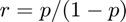$r = p / (1-p)$ . Higher odds indicates a higher probability of observing a one.

rng(7639)
nc3 = 3; % Number of components
sz3 = [50 60 70]; % Tensor size
nd3 = length(sz3); % Number of dimensions

We assume that the underlying model tensor has factor matrices with only a few "large" entries in each column. The small entries should correspond to a low but nonzero entry of observing a 1, while the largest entries, if multiplied together, should correspond to a very high likelihood of observing a 1.

probrange = [0.01 0.99]; % Absolute min and max of probabilities
oddsrange = probrange ./ (1 - probrange);
smallval = nthroot(min(oddsrange)/nc3,nd3);
largeval = nthroot(max(oddsrange)/nc3,nd3);

A3 = cell(nd3,1);
for k = 1:nd3
    A3{k} = smallval * ones(sz3(k), nc3);
    nbig = 5;
    for j = 1:nc3
        p = randperm(sz3(k));
        A3{k}(p(1:nbig),j) = largeval;
    end
end
M3_true = ktensor(A3);
clear probrange oddsrange smallval largeval nbig p A3;

Convert K-tensor to an observed tensor Get the model values, which correspond to odds of observing a 1

Mfull3 = full(M3_true);
% Convert odds to probabilities
Mprobs3 = Mfull3 ./ (1 + Mfull3);
% Flip a coin for each entry, with the probability of observing a one
% dictated by Mprobs
rng('default');
Xfull3 = 1.0*(tensor(@rand, sz3) < Mprobs3);
% Convert to sparse tensor, real-valued 0/1 tensor since it was constructed
% to be sparse
X3 = sptensor(Xfull3);
fprintf('Proportion of nonzeros in X is %.2f%%\n', 100*nnz(X3) / prod(sz3));

Proportion of nonzeros in X is 8.39%

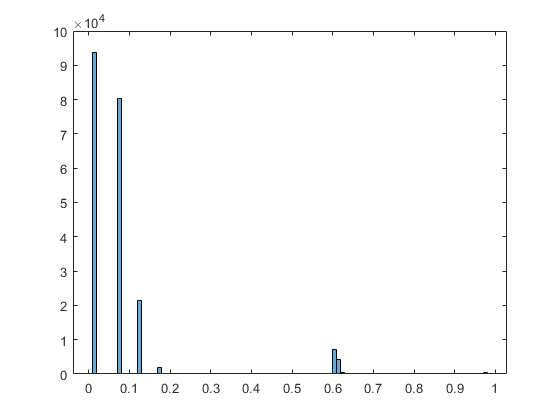
Just for fun, let's visualize the distribution of the probabilities in the model tensor.

histogram(Mprobs3(:))

Call GCP_OPT on the full tensor. Here we specify tighter tolerances.

rng('default');
M3_1 = gcp_opt(Xfull3, nc3, 'type', 'binary', 'printitn', 25, 'pgtol', 1e-6, 'factr', 1e4);
fprintf('Final score: %f\n', score(M3_1,M3_true));

GCP-OPT-LBFGSB (Generalized CP Tensor Decomposition)

Tensor size: 50 x 60 x 70 (210000 total entries)
GCP rank: 3
Generalized function Type: binary
Objective function: @(x,m)log(m+1)-x.*log(m+1e-10)
Gradient function: @(x,m)1./(m+1)-x./(m+1e-10)
Lower bound of factor matrices: 0
Optimization method: lbfgsb
Max iterations: 1000
Projected gradient tolerance: 1e-06

Begin Main loop
Iter    25, f(x) = 4.658479e+04, ||grad||_infty = 6.05e+01
Iter    50, f(x) = 4.467162e+04, ||grad||_infty = 6.94e+01
Iter    75, f(x) = 4.336750e+04, ||grad||_infty = 5.78e+01
Iter   100, f(x) = 4.331052e+04, ||grad||_infty = 1.07e+01
Iter   125, f(x) = 4.330680e+04, ||grad||_infty = 1.11e+00
Iter   150, f(x) = 4.330667e+04, ||grad||_infty = 2.39e-01
Iter   175, f(x) = 4.330666e+04, ||grad||_infty = 2.51e-02
Iter   194, f(x) = 4.330666e+04, ||grad||_infty = 3.07e-03
End Main Loop

Final objective: 4.3307e+04
Setup time: 0.00 seconds
Main loop time: 1.66 seconds
Outer iterations: 194
Total iterations: 407
L-BFGS-B Exit message: CONVERGENCE: REL_REDUCTION_OF_F_<=_FACTR*EPSMCH.
Final score: 0.894842

GCP-OPT as sparse tensor

rng('default');
M3_2 = gcp_opt(X3, nc3, 'type', 'binary');
fprintf('Final score: %f\n', score(M3_2,M3_true));

GCP-OPT-ADAM (Generalized CP Tensor Decomposition)

Tensor size: 50 x 60 x 70 (210000 total entries)
Sparse tensor: 17613 (8.4%) Nonzeros and 192387 (91.61%) Zeros
GCP rank: 3
Generalized function Type: binary
Objective function: @(x,m)log(m+1)-x.*log(m+1e-10)
Gradient function: @(x,m)1./(m+1)-x./(m+1e-10)
Lower bound of factor matrices: 0
Optimization method: adam
Max iterations (epochs): 1000
Iterations per epoch: 1000
Learning rate / decay / maxfails: 0.001 0.1 1
Function Sampler: stratified with 17613 nonzero and 17613 zero samples
Gradient Sampler: stratified with 1000 nonzero and 1000 zero samples

Begin Main loop
Initial f-est: 7.186598e+04
Epoch  1: f-est = 4.749859e+04, step = 0.001
Epoch  2: f-est = 4.695772e+04, step = 0.001
Epoch  3: f-est = 4.675392e+04, step = 0.001
Epoch  4: f-est = 4.625718e+04, step = 0.001
Epoch  5: f-est = 4.557864e+04, step = 0.001
Epoch  6: f-est = 4.529161e+04, step = 0.001
Epoch  7: f-est = 4.512106e+04, step = 0.001
Epoch  8: f-est = 4.492460e+04, step = 0.001
Epoch  9: f-est = 4.429687e+04, step = 0.001
Epoch 10: f-est = 4.370145e+04, step = 0.001
Epoch 11: f-est = 4.356684e+04, step = 0.001
Epoch 12: f-est = 4.350982e+04, step = 0.001
Epoch 13: f-est = 4.352045e+04, step = 0.001, nfails = 1 (resetting to solution from last epoch)
Epoch 14: f-est = 4.349492e+04, step = 0.0001
Epoch 15: f-est = 4.348921e+04, step = 0.0001
Epoch 16: f-est = 4.348955e+04, step = 0.0001, nfails = 2 (resetting to solution from last epoch)
End Main Loop

Final f-est: 4.3489e+04
Setup time: 0.01 seconds
Main loop time: 10.88 seconds
Total iterations: 16000
Final score: 0.784293

Create and test a Poisson count tensor.

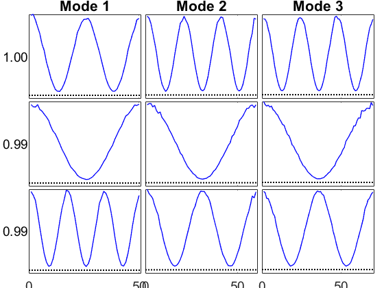
nc4 = 3;
sz4 = [80 90 100];
nd4 = length(sz4);
paramRange = [0.5 60];
factorRange = paramRange.^(1/nd4);
minFactorRatio = 95/100;
lambdaDamping = 0.8;
rng(21);
info4 = create_problem('Size', sz4, ...
    'Num_Factors', nc4, ...
    'Factor_Generator', @(m,n)factorRange(1)+(rand(m,n)>minFactorRatio)*(factorRange(2)-factorRange(1)), ...
    'Lambda_Generator', @(m,n)ones(m,1)*(lambdaDamping.^(0:n-1)'), ...
    'Sparse_Generation', 0.2);

M4_true = normalize(arrange(info4.Soln));
X4 = info4.Data;
viz(M4_true, 'Figure',4);
clear paramRange factorRange minFactorRatio lambdaDamping;

ktensor/viz: Normalizing factors and sorting components according to the 2-norm.

Loss function for Poisson negative log likelihood with identity link.

% Call GCP_OPT on sparse tensor
rng('default');
M4 = gcp_opt(X4, nc4, 'type', 'count','printitn',25);
fprintf('Final score: %f\n', score(M4,M4_true));

GCP-OPT-ADAM (Generalized CP Tensor Decomposition)

Tensor size: 80 x 90 x 100 (720000 total entries)
Sparse tensor: 123856 (17%) Nonzeros and 596144 (82.80%) Zeros
GCP rank: 3
Generalized function Type: count
Objective function: @(x,m)m-x.*log(m+1e-10)
Gradient function: @(x,m)1-x./(m+1e-10)
Lower bound of factor matrices: 0
Optimization method: adam
Max iterations (epochs): 1000
Iterations per epoch: 1000
Learning rate / decay / maxfails: 0.001 0.1 1
Function Sampler: stratified with 100000 nonzero and 100000 zero samples
Gradient Sampler: stratified with 1000 nonzero and 1000 zero samples

Begin Main loop
Initial f-est: 4.702050e+05
Epoch 12: f-est = 3.448229e+05, step = 0.001, nfails = 1 (resetting to solution from last epoch)
Epoch 16: f-est = 3.447395e+05, step = 0.0001, nfails = 2 (resetting to solution from last epoch)
End Main Loop

Final f-est: 3.4473e+05
Setup time: 0.04 seconds
Main loop time: 14.02 seconds
Total iterations: 16000
Final score: 0.951592