
Kruskal Tensors
Kruskal format is a decomposition of a tensor X as the sum of the outer products as the columns of matrices. For example, we might write
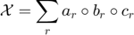
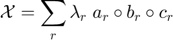
where a subscript denotes column index and a circle denotes outer product. In other words, the tensor X is built from the columns of the matrices A,B, and C. It's often helpful to explicitly specify a weight for each outer product, which we do here:
The ktensor class stores the components of the tensor X and can perform many operations, e.g., ttm, without explicitly forming the tensor X.
Contents
- Kruskal tensor format via ktensor
- Specifying weights in a ktensor
- Creating a one-dimensional ktensor
- Constituent parts of a ktensor
- Creating a ktensor from its constituent parts
- Creating an empty ktensor
- Use full or tensor to convert a ktensor to a tensor
- Use double to convert a ktensor to a multidimensional array
- Use tendiag or sptendiag to convert a ktensor to a ttensor.
- Use ndims and size for the dimensions of a ktensor
- Subscripted reference for a ktensor
- Subscripted assignment for a ktensor
- Use end for the last array index.
- Adding and subtracting ktensors
- Basic operations with a ktensor
- Use permute to reorder the modes of a ktensor
- Use arrange to normalize the factors of a ktensor
- Use fixsigns for sign indeterminacies in a ktensor
- Use ktensor to store the 'skinny' SVD of a matrix
- Displaying a ktensor
- Displaying data
Kruskal tensor format via ktensor
Kruskal format stores a tensor as a sum of rank-1 outer products. For example, consider a tensor of the following form.

This can be stored in Kruskal form as follows.
rand('state',0);
A = rand(4,2); %<-- First column is a_1, second is a_2.
B = rand(3,2); %<-- Likewise for B.
C = rand(2,2); %<-- Likewise for C.
X = ktensor({A,B,C}) %<-- Create the ktensor.
X is a ktensor of size 4 x 3 x 2
	X.lambda =
		     1     1
	X.U{1} =
		    0.9501    0.8913
		    0.2311    0.7621
		    0.6068    0.4565
		    0.4860    0.0185
	X.U{2} =
		    0.8214    0.7919
		    0.4447    0.9218
		    0.6154    0.7382
	X.U{3} =
		    0.1763    0.9355
		    0.4057    0.9169
For Kruskal format, there can be any number of matrices, but every matrix must have the same number of columns. The number of rows can vary.
Y = ktensor({rand(4,1),rand(2,1),rand(3,1)}) %<-- Another ktensor.
Y is a ktensor of size 4 x 2 x 3
	Y.lambda =
		     1
	Y.U{1} =
		    0.4103
		    0.8936
		    0.0579
		    0.3529
	Y.U{2} =
		    0.8132
		    0.0099
	Y.U{3} =
		    0.1389
		    0.2028
		    0.1987
Specifying weights in a ktensor
Weights for each rank-1 tensor can be specified by passing in a column vector. For example,

lambda = [5.0; 0.25]; %<-- Weights for each factor.
X = ktensor(lambda,{A,B,C}) %<-- Create the ktensor.
X is a ktensor of size 4 x 3 x 2
	X.lambda =
		    5.0000    0.2500
	X.U{1} =
		    0.9501    0.8913
		    0.2311    0.7621
		    0.6068    0.4565
		    0.4860    0.0185
	X.U{2} =
		    0.8214    0.7919
		    0.4447    0.9218
		    0.6154    0.7382
	X.U{3} =
		    0.1763    0.9355
		    0.4057    0.9169
Creating a one-dimensional ktensor
Y = ktensor({rand(4,5)}) %<-- A one-dimensional ktensor.
Y is a ktensor of size 4
	Y.lambda =
		     1     1     1     1     1
	Y.U{1} =
		    0.6038    0.7468    0.4186    0.6721    0.3795
		    0.2722    0.4451    0.8462    0.8381    0.8318
		    0.1988    0.9318    0.5252    0.0196    0.5028
		    0.0153    0.4660    0.2026    0.6813    0.7095
Constituent parts of a ktensor
X.lambda %<-- Weights or multipliers.
ans =

    5.0000
    0.2500
X.U %<-- Cell array of matrices.
ans =

  3×1 cell array

    {4×2 double}
    {3×2 double}
    {2×2 double}
Creating a ktensor from its constituent parts
Y = ktensor(X.lambda,X.U) %<-- Recreate X.
Y is a ktensor of size 4 x 3 x 2
	Y.lambda =
		    5.0000    0.2500
	Y.U{1} =
		    0.9501    0.8913
		    0.2311    0.7621
		    0.6068    0.4565
		    0.4860    0.0185
	Y.U{2} =
		    0.8214    0.7919
		    0.4447    0.9218
		    0.6154    0.7382
	Y.U{3} =
		    0.1763    0.9355
		    0.4057    0.9169
Creating an empty ktensor
Z = ktensor %<-- Empty ktensor.
Z is a ktensor of size [empty tensor]
	Z.lambda =
Use full or tensor to convert a ktensor to a tensor
full(X) %<-- Converts to a tensor.
ans is a tensor of size 4 x 3 x 2
	ans(:,:,1) =
	    0.8529    0.5645    0.6692
	    0.3085    0.2549    0.2569
	    0.5239    0.3362    0.4080
	    0.3552    0.1945    0.2668
	ans(:,:,2) =
	    1.7450    1.0454    1.3370
	    0.5235    0.3695    0.4175
	    1.0940    0.6439    0.8348
	    0.8131    0.4423    0.6098
tensor(X) %<-- Same as above.
ans is a tensor of size 4 x 3 x 2
	ans(:,:,1) =
	    0.8529    0.5645    0.6692
	    0.3085    0.2549    0.2569
	    0.5239    0.3362    0.4080
	    0.3552    0.1945    0.2668
	ans(:,:,2) =
	    1.7450    1.0454    1.3370
	    0.5235    0.3695    0.4175
	    1.0940    0.6439    0.8348
	    0.8131    0.4423    0.6098
Use double to convert a ktensor to a multidimensional array
double(X) %<-- Converts to an array.
ans(:,:,1) =
    0.8529    0.5645    0.6692
    0.3085    0.2549    0.2569
    0.5239    0.3362    0.4080
    0.3552    0.1945    0.2668
ans(:,:,2) =
    1.7450    1.0454    1.3370
    0.5235    0.3695    0.4175
    1.0940    0.6439    0.8348
    0.8131    0.4423    0.6098
Use tendiag or sptendiag to convert a ktensor to a ttensor.
A ktensor can be regarded as a ttensor with a diagonal core.
R = length(X.lambda);  %<-- Number of factors in X.
core = tendiag(X.lambda, repmat(R,1,ndims(X))); %<-- Create a diagonal core.
Y = ttensor(core, X.u) %<-- Assemble the ttensor.
Y is a ttensor of size 4 x 3 x 2
	Y.core is a tensor of size 2 x 2 x 2
		Y.core(:,:,1) =
	     5     0
	     0     0
		Y.core(:,:,2) =
	         0         0
	         0    0.2500
	Y.U{1} =
		    0.9501    0.8913
		    0.2311    0.7621
		    0.6068    0.4565
		    0.4860    0.0185
	Y.U{2} =
		    0.8214    0.7919
		    0.4447    0.9218
		    0.6154    0.7382
	Y.U{3} =
		    0.1763    0.9355
		    0.4057    0.9169
norm(full(X)-full(Y)) %<-- They are the same.
ans =
   3.7238e-16
core = sptendiag(X.lambda, repmat(R,1,ndims(X))); %<-- Sparse diagonal core.
Y = ttensor(core, X.u) %<-- Assemble the ttensor
Y is a ttensor of size 4 x 3 x 2
	Y.core is a sparse tensor of size 2 x 2 x 2 with 2 nonzeros
	(1,1,1)    5.0000
	(2,2,2)    0.2500
	Y.U{1} =
		    0.9501    0.8913
		    0.2311    0.7621
		    0.6068    0.4565
		    0.4860    0.0185
	Y.U{2} =
		    0.8214    0.7919
		    0.4447    0.9218
		    0.6154    0.7382
	Y.U{3} =
		    0.1763    0.9355
		    0.4057    0.9169
norm(full(X)-full(Y)) %<-- They are the same.
ans =
   3.7238e-16
Use ndims and size for the dimensions of a ktensor
ndims(X) %<-- Number of dimensions.
ans =
     3
size(X) %<-- Row vector of the sizes.
ans =
     4     3     2
size(X,2) %<-- Size of the 2nd mode.
ans =
     3
Subscripted reference for a ktensor
X(1,1,1) %<-- Assemble the (1,1,1) element (requires computation).
ans =
    0.8529
X.lambda(2) %<-- Weight of 2nd factor.
ans =
    0.2500
X.U{2} %<-- Extract a matrix.
ans =
    0.8214    0.7919
    0.4447    0.9218
    0.6154    0.7382
X{2} %<-- Same as above.
ans =
    0.8214    0.7919
    0.4447    0.9218
    0.6154    0.7382
Subscripted assignment for a ktensor
X.lambda = ones(size(X.lambda)) %<-- Insert new multipliers.
X is a ktensor of size 4 x 3 x 2
	X.lambda =
		     1     1
	X.U{1} =
		    0.9501    0.8913
		    0.2311    0.7621
		    0.6068    0.4565
		    0.4860    0.0185
	X.U{2} =
		    0.8214    0.7919
		    0.4447    0.9218
		    0.6154    0.7382
	X.U{3} =
		    0.1763    0.9355
		    0.4057    0.9169
X.lambda(1) = 7 %<-- Change a single element of lambda.
X is a ktensor of size 4 x 3 x 2
	X.lambda =
		     7     1
	X.U{1} =
		    0.9501    0.8913
		    0.2311    0.7621
		    0.6068    0.4565
		    0.4860    0.0185
	X.U{2} =
		    0.8214    0.7919
		    0.4447    0.9218
		    0.6154    0.7382
	X.U{3} =
		    0.1763    0.9355
		    0.4057    0.9169
X{3}(1:2,1) = [1;1] %<-- Change the matrix for mode 3.
X is a ktensor of size 4 x 3 x 2
	X.lambda =
		     7     1
	X.U{1} =
		    0.9501    0.8913
		    0.2311    0.7621
		    0.6068    0.4565
		    0.4860    0.0185
	X.U{2} =
		    0.8214    0.7919
		    0.4447    0.9218
		    0.6154    0.7382
	X.U{3} =
		    1.0000    0.9355
		    1.0000    0.9169
Use end for the last array index.
X(3:end,1,1) %<-- Calculated X(3,1,1) and X((4,1,1).
ans =
    3.8274
    2.8080
X(1,1,1:end-1) %<-- Calculates X(1,1,1).
ans =
    6.1234
X{end} %<-- Or use inside of curly braces. This is X{3}.
ans =
    1.0000    0.9355
    1.0000    0.9169
Adding and subtracting ktensors
Adding two ktensors is the same as concatenating the matrices
X = ktensor({rand(4,2),rand(2,2),rand(3,2)}) %<-- Data.
Y = ktensor({rand(4,2),rand(2,2),rand(3,2)}) %<-- More data.
X is a ktensor of size 4 x 2 x 3
	X.lambda =
		     1     1
	X.U{1} =
		    0.4289    0.6822
		    0.3046    0.3028
		    0.1897    0.5417
		    0.1934    0.1509
	X.U{2} =
		    0.6979    0.8600
		    0.3784    0.8537
	X.U{3} =
		    0.5936    0.8216
		    0.4966    0.6449
		    0.8998    0.8180
Y is a ktensor of size 4 x 2 x 3
	Y.lambda =
		     1     1
	Y.U{1} =
		    0.6602    0.5341
		    0.3420    0.7271
		    0.2897    0.3093
		    0.3412    0.8385
	Y.U{2} =
		    0.5681    0.7027
		    0.3704    0.5466
	Y.U{3} =
		    0.4449    0.7948
		    0.6946    0.9568
		    0.6213    0.5226
Z = X + Y %<-- Concatenates the factor matrices.
Z is a ktensor of size 4 x 2 x 3
	Z.lambda =
		     1     1     1     1
	Z.U{1} =
		    0.4289    0.6822    0.6602    0.5341
		    0.3046    0.3028    0.3420    0.7271
		    0.1897    0.5417    0.2897    0.3093
		    0.1934    0.1509    0.3412    0.8385
	Z.U{2} =
		    0.6979    0.8600    0.5681    0.7027
		    0.3784    0.8537    0.3704    0.5466
	Z.U{3} =
		    0.5936    0.8216    0.4449    0.7948
		    0.4966    0.6449    0.6946    0.9568
		    0.8998    0.8180    0.6213    0.5226
Z = X - Y %<-- Concatenates as with plus, but changes the weights.
Z is a ktensor of size 4 x 2 x 3
	Z.lambda =
		     1     1    -1    -1
	Z.U{1} =
		    0.4289    0.6822    0.6602    0.5341
		    0.3046    0.3028    0.3420    0.7271
		    0.1897    0.5417    0.2897    0.3093
		    0.1934    0.1509    0.3412    0.8385
	Z.U{2} =
		    0.6979    0.8600    0.5681    0.7027
		    0.3784    0.8537    0.3704    0.5466
	Z.U{3} =
		    0.5936    0.8216    0.4449    0.7948
		    0.4966    0.6449    0.6946    0.9568
		    0.8998    0.8180    0.6213    0.5226
norm( full(Z) - (full(X)-full(Y)) ) %<-- Should be zero.
ans =
   1.8968e-16
Basic operations with a ktensor
+X %<-- Calls uplus.
ans is a ktensor of size 4 x 2 x 3
	ans.lambda =
		     1     1
	ans.U{1} =
		    0.4289    0.6822
		    0.3046    0.3028
		    0.1897    0.5417
		    0.1934    0.1509
	ans.U{2} =
		    0.6979    0.8600
		    0.3784    0.8537
	ans.U{3} =
		    0.5936    0.8216
		    0.4966    0.6449
		    0.8998    0.8180
-X %<-- Calls uminus.
ans is a ktensor of size 4 x 2 x 3
	ans.lambda =
		    -1    -1
	ans.U{1} =
		    0.4289    0.6822
		    0.3046    0.3028
		    0.1897    0.5417
		    0.1934    0.1509
	ans.U{2} =
		    0.6979    0.8600
		    0.3784    0.8537
	ans.U{3} =
		    0.5936    0.8216
		    0.4966    0.6449
		    0.8998    0.8180
5*X %<-- Calls mtimes.
ans is a ktensor of size 4 x 2 x 3
	ans.lambda =
		     5     5
	ans.U{1} =
		    0.4289    0.6822
		    0.3046    0.3028
		    0.1897    0.5417
		    0.1934    0.1509
	ans.U{2} =
		    0.6979    0.8600
		    0.3784    0.8537
	ans.U{3} =
		    0.5936    0.8216
		    0.4966    0.6449
		    0.8998    0.8180
Use permute to reorder the modes of a ktensor
permute(X,[2 3 1]) %<-- Reorders modes of X
ans is a ktensor of size 2 x 3 x 4
	ans.lambda =
		     1     1
	ans.U{1} =
		    0.6979    0.8600
		    0.3784    0.8537
	ans.U{2} =
		    0.5936    0.8216
		    0.4966    0.6449
		    0.8998    0.8180
	ans.U{3} =
		    0.4289    0.6822
		    0.3046    0.3028
		    0.1897    0.5417
		    0.1934    0.1509
Use arrange to normalize the factors of a ktensor
The function arrange normalizes the columns of the factors and then arranges the rank-one pieces in decreasing order of size.
X = ktensor({rand(3,2),rand(4,2),rand(2,2)}) % <-- Unit weights.
X is a ktensor of size 3 x 4 x 2
	X.lambda =
		     1     1
	X.U{1} =
		    0.8801    0.2714
		    0.1730    0.2523
		    0.9797    0.8757
	X.U{2} =
		    0.7373    0.1991
		    0.1365    0.2987
		    0.0118    0.6614
		    0.8939    0.2844
	X.U{3} =
		    0.4692    0.9883
		    0.0648    0.5828
arrange(X) %<-- Normalized and rearranged.
ans is a ktensor of size 3 x 4 x 2
	ans.lambda =
		    0.8778    0.7342
	ans.U{1} =
		    0.2855    0.6626
		    0.2653    0.1302
		    0.9209    0.7376
	ans.U{2} =
		    0.2475    0.6319
		    0.3713    0.1170
		    0.8221    0.0101
		    0.3535    0.7661
	ans.U{3} =
		    0.8614    0.9906
		    0.5079    0.1368
Use fixsigns for sign indeterminacies in a ktensor
The largest magnitude entry for each factor is changed to be positive provided that we can flip the signs of pairs of vectors in that rank-1 component.
Y = X;
Y.u{1}(:,1) = -Y.u{1}(:,1);  % switch the sign on a pair of columns
Y.u{2}(:,1) = -Y.u{2}(:,1)
Y is a ktensor of size 3 x 4 x 2
	Y.lambda =
		     1     1
	Y.U{1} =
		   -0.8801    0.2714
		   -0.1730    0.2523
		   -0.9797    0.8757
	Y.U{2} =
		   -0.7373    0.1991
		   -0.1365    0.2987
		   -0.0118    0.6614
		   -0.8939    0.2844
	Y.U{3} =
		    0.4692    0.9883
		    0.0648    0.5828
fixsigns(Y)
ans is a ktensor of size 3 x 4 x 2
	ans.lambda =
		     1     1
	ans.U{1} =
		    0.8801    0.2714
		    0.1730    0.2523
		    0.9797    0.8757
	ans.U{2} =
		    0.7373    0.1991
		    0.1365    0.2987
		    0.0118    0.6614
		    0.8939    0.2844
	ans.U{3} =
		    0.4692    0.9883
		    0.0648    0.5828
Use ktensor to store the 'skinny' SVD of a matrix
A = rand(4,3) %<-- A random matrix.
A =
    0.4235    0.2259    0.6405
    0.5155    0.5798    0.2091
    0.3340    0.7604    0.3798
    0.4329    0.5298    0.7833
[U,S,V] = svd(A,0); %<-- Compute the SVD.
X = ktensor(diag(S),{U,V}) %<-- Store the SVD as a ktensor.
X is a ktensor of size 4 x 3
	X.lambda =
		    1.7002    0.5095    0.2277
	X.U{1} =
		   -0.4346   -0.5816    0.3635
		   -0.4365    0.5184    0.6947
		   -0.5109    0.4983   -0.5366
		   -0.5996   -0.3804   -0.3120
	X.U{2} =
		   -0.4937    0.0444    0.8685
		   -0.6220    0.6800   -0.3883
		   -0.6078   -0.7319   -0.3080
double(X) %<-- Reassemble the original matrix.
ans =
    0.4235    0.2259    0.6405
    0.5155    0.5798    0.2091
    0.3340    0.7604    0.3798
    0.4329    0.5298    0.7833
Displaying a ktensor
disp(X) %<-- Displays the vector lambda and each factor matrix.
ans is a ktensor of size 4 x 3
	ans.lambda =
		    1.7002    0.5095    0.2277
	ans.U{1} =
		   -0.4346   -0.5816    0.3635
		   -0.4365    0.5184    0.6947
		   -0.5109    0.4983   -0.5366
		   -0.5996   -0.3804   -0.3120
	ans.U{2} =
		   -0.4937    0.0444    0.8685
		   -0.6220    0.6800   -0.3883
		   -0.6078   -0.7319   -0.3080
Displaying data
The datadisp function allows the user to associate meaning to the modes and display those modes with the most meaning (i.e., corresponding to the largest values).
X = ktensor({[0.8 0.1 1e-10]',[1e-5 2 3 1e-4]',[0.5 0.5]'}); %<-- Create tensor.
X = arrange(X) %<-- Normalize the factors.
X is a ktensor of size 3 x 4 x 2
	X.lambda =
		    2.0555
	X.U{1} =
		    0.9923
		    0.1240
		    0.0000
	X.U{2} =
		    0.0000
		    0.5547
		    0.8321
		    0.0000
	X.U{3} =
		    0.7071
		    0.7071
labelsDim1 = {'one','two','three'}; %<-- Labels for mode 1.
labelsDim2 = {'A','B','C','D'}; %<-- Labels for mode 2.
labelsDim3 = {'on','off'}; %<-- Labels for mode 3.
datadisp(X,{labelsDim1,labelsDim2,labelsDim3}) %<-- Display.
======== Group 1 ========

Weight = 2.055480
Score      Id   Name
 0.9922779     1 one
 0.1240347     2 two
Score      Id   Name
 0.8320503     3 C
 0.5547002     2 B
 2.774e-05     4 D
 2.774e-06     1 A
Score      Id   Name
 0.7071068     1 on
 0.7071068     2 off